We show on several examples the features of this new function. Note that all the following examples are based on simulated data set.
In each case (except if the converse is specified), we give as one of the inputs, the true proportions (i.e the proportions which have been used to simulate the facies).
List of the examples:
1) Mono-Gaussian case with stationary proportions (1D)
2) Mono-Gaussian case with non-stationary proportions (1D)
a) Gaussian covariance function
b) Exponential covariance function
3) Bi-Gaussian case with stationary proportions
Example 1: mono-Gaussian case with stationary proportions
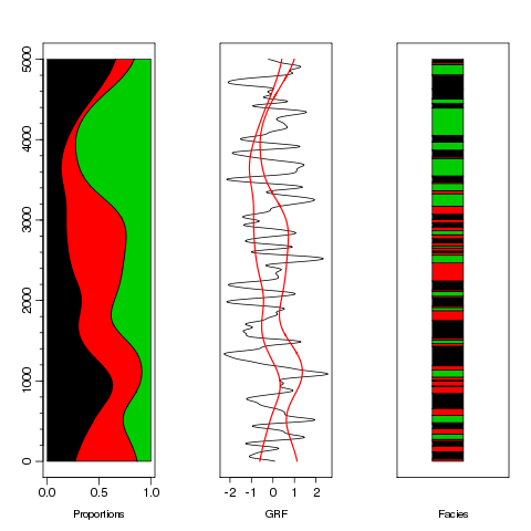
In this example in 1D, we work with only one GRF and three facies with identical proportions.
First, we have to create the model of the GRF, the rule object (see related tutorial) and to simulate the data.
Before threshing the GRF, we compute its variogram for comparison purposes.
- Code: Select all
model=model.create(vartype="Gaussian",range=100,ndim=1)
rule = rule.create(c("S","F1","S","F2","F3"))
db=db.create(nx=5000)
db=simtub(dbout=db,model=model,nbtuba=2000)
vario_exp=vario.grid(db,nlag=200)
db=db.rule(db,rule=rule)
We can display the rule:
- Code: Select all
plot(rule)

We can display the data:
- Code: Select all
par(mfrow=c(1,3))

plot(c(0,1),c(1,5000),cex=0,xlab="Proportions",ylab="",xaxp=c(0,1,2),yaxp=c(0,5000,5),cex.lab=1.2,cex.axis=1.4,tcl=-.7)
axis(2,at=1:25*200,label=F,tcl=-.3)
polygon(c(0,1/3,1/3,0),c(1,1,5000,5000),col=1)
polygon(c(1/3,2/3,2/3,1/3),c(1,1,5000,5000),col=2)
polygon(c(2/3,1,1,2/3),c(1,1,5000,5000),col=3)

plot(db[,3],1:5000,type="l",yaxt="n",xlab="GRF",cex.lab=1.2,cex.axis=1.4,ylab="")
abline(v=c(qnorm(1/3),qnorm(2/3)),col=2,lwd=1.5)
from=c(1,.5+(1:4999)[db[-1,4]!=db[-5000,4]],5000)

plot(c(0,1),c(1,5000),cex=0,xlab="Facies",ylab="",xaxt="n",yaxt="n",cex.lab=1.2,cex.axis=1.4)
cols=c(db[1,4],db[-1,][db[-1,4]!=db[-5000,4],4])
for(i in 1:(length(from)-1))
polygon(c(.3,.6,.6,.3),c(from[i],from[i],from[i+1],from[i+1]),col=cols[i])

And now we compute the experimental variogram with the vario.pgs method (for 200 lags of size 1)
- Code: Select all
vario=vario.pgs(db,rule=rule,lag=1,nlag=200,calcul="vg")
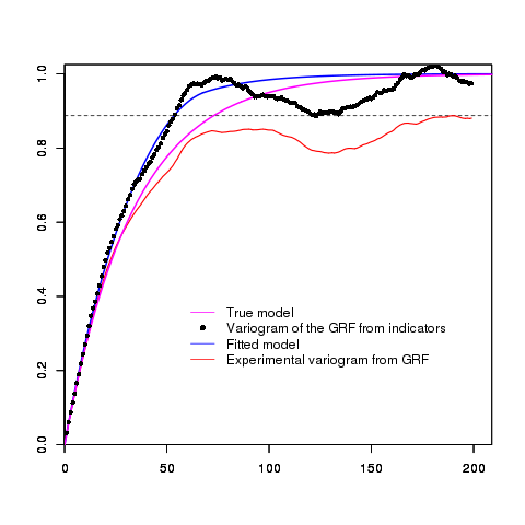
We can now fit the obtained experimental variogram and display the results:
- Code: Select all
par(omi=rep(0,4))
model_fit=model.auto(vario,flag.norm.sill=T,draw=F)
plot(vario_exp,col=2,lwd=1.5)
legend(60,.4,legend=c("True model","Variogram of the GRF from indicators","Fitted model","Experimental variogram from GRF"),
col=c(6,1,4,2),lty=c(1,NA,1,1),pch=c(NA,16,NA,NA),box.col=0)
plot(model_fit,add=T,col=4,vario=vario)
plot(model,col=6,add=T,vario=vario)
points(vario[1]$hh,vario[1]$gg,cex=.8,pch=16)

As we can see, the variogram otained by vario.pgs from the facies data is very close to the experimental variogram computed on the realization of the GRF (red) although some information has been lost by the truncation.
Example 2:
mono-Gaussian case with non-stationary proportions
Case 1 - Gaussian covariance
In this example in 1D, we work with only one GRF and three facies with varying proportions.
First, we have to create the model of the GRF, the rule object and to simulate the data.
Before threshing the GRF, we compute its variogram for comparison purposes.
- Code: Select all
model=model.create(vartype="Gaussian",range=100,ndim=1)
rule = rule.create(c("S","F1","S","F2","F3"))
db=db.create(nx=5000)
db=simtub(dbout=db,model=model,nbtuba=2000)
vario_exp=vario.grid(db,nlag=200)
model.prop=model.create(vartype="Gaussian",range=1000,ndim=1)
db.prop=db.create(nx=5000)
db.prop=simtub(dbout=db.prop,model=model.prop,seed=12213,nbtuba=2000,nbsimu=3)
proportions=exp(db.prop[,3:4])/(apply(exp(db.prop[,3:4]),1,sum)+1)
proportions=cbind(proportions,1-apply(proportions[,1:2],1,sum))
db=db.add(db,proportions,locnames=c("p1","p2","p3"))
db=db.rule(db,rule=rule)
We can display the data:
- Code: Select all
par(mfrow=c(1,3))

plot(c(0,1),c(1,5000),cex=0,xlab="Proportions",ylab="",xaxp=c(0,1,2),yaxp=c(0,5000,5),cex.lab=1.2,cex.axis=1.4,tcl=-.7)
axis(2,at=1:25*200,label=F,tcl=-.3)
polygon(c(0,db[,4],0),c(1,1:5000,5000),col=1)
polygon(c(db[5000:1,4],1-db[,6]),c(5000:1,1:5000),col=2)
polygon(c(1-db[,6],1,1),c(1:5000,5000,1),col=3)

plot(db[,3],1:5000,type="l",yaxt="n",xlab="GRF",cex.lab=1.2,cex.axis=1.4,ylab="")
lines(qnorm(db[,4]),1:5000,col=2,lwd=1.5)
lines(qnorm(1-db[,6]),1:5000,col=2,lwd=1.5)
from=c(1,.5+(1:4999)[db[-1,7]!=db[-5000,7]],5000)

plot(c(0,1),c(1,5000),cex=0,xlab="Facies",ylab="",xaxt="n",yaxt="n",cex.lab=1.2,cex.axis=1.4)
cols=c(db[1,7],db[-1,][db[-1,7]!=db[-5000,7],7])
for(i in 1:(length(from)-1))
polygon(c(.3,.6,.6,.3),c(from[i],from[i],from[i+1],from[i+1]),col=cols[i])
And now we compute the experimental variogram with the vario.pgs method (for 200 lags of size 1). The proportions are taken into account as they are in the db with locators p.
It is more time consuming since the non-stationarity of the proportions!
- Code: Select all
vario=vario.pgs(db,rule=rule,lag=1,nlag=200,calcul="vg")
We can now fit the obtained experimental variogram and display the results:
- Code: Select all
par(omi=rep(0,4))
model_fit=model.auto(vario,flag.norm.sill=T,draw=F)
plot(vario_exp,col=2,lwd=1.5)
legend(60,.4,legend=c("True model","Variogram of the GRF from indicators","Fitted model","Experimental variogram from GRF"),
col=c(6,1,4,2),lty=c(1,NA,1,1),pch=c(NA,16,NA,NA),box.col=0)
plot(model_fit,add=T,col=4,vario=vario)
plot(model,col=6,add=T,vario=vario)
points(vario[1]$hh,vario[1]$gg,cex=.8,pch=16)

Case 2 - Exponential covariance
In this example, we apply exactly the same code as previously but we use an
Exponential basic structure instead of a Gaussian one:
- Code: Select all
model=model.create(vartype="Exponential",range=100,ndim=1)
We display the data:

and the results
Example 3:
Bi-Gaussian case with stationary proportions
In this exemple (in 2D), the 3 facies are defined by using two independent GRF's according to the following rule :
- Code: Select all
data(Exdemo_simpgs_std.rule)
plot(Exdemo_simpgs_std.rule)

Then,
- 1) we simulate the 2 independent GRFs (the first one with a Gaussian covariance structure and the second one with an Exponential one)
2) we compute their experimental variograms (for comparison purpose)
3) we create the facies variable by threshing the GRFs according to the rule.
4) the data are displayed.
- Code: Select all
set.seed(234)
data(Exdemo_simpgs_std.rule)
db=db.create(x1=runif(1000),x2=runif(1000),ndim=2)
model1=model.create(vartype="Gaussian",range=.2,ndim=2)
model2=model.create(vartype="Exponential",range=.3,ndim=2)
db=simtub(dbout=db,model=model1,nbtuba=2000)
vario_exp1=vario.calc(db,nlag=30)
db=simtub(dbout=db,model=model2,nbtuba=2000)
vario_exp2=vario.calc(db,nlag=30)
db=db.locate(db,4:5,"z")
db=db.rule(db,rule=Exdemo_simpgs_std.rule)
plot(db[,2],db[,3],col=db[,6],pch=16,xlab="",ylab="",cex=.6)
title("Data: 3 categories")

We then compute the experimental variograms (30 lags) by using vario.pgs:
- Code: Select all
vario=vario.pgs(db,rule=Exdemo_simpgs_std.rule,nlag=30)
We extract the first simple variogram of the bivariate one and then display the results:
- Code: Select all
v1=vario.reduce(vario=vario,vars=1,flag.vario=TRUE)
model_fit=model.auto(v1,flag.norm.sill=T,draw=F)
plot(vario_exp1,col=2,lwd=1.5,ylab=expression(gamma))
legend(0.2,.6,legend=c("True model","Variogram of the GRF from indicators","Fitted model","Experimental variogram from GRF"),
col=c(6,1,4,2),lty=c(1,NA,1,1),pch=c(NA,16,NA,NA),box.col=0)
plot(model_fit,add=T,col=4,vario=v1)
plot(model1,col=6,add=T,vario=v1)
points(v1[1]$hh,v1[1]$gg,cex=.8,pch=16)

We do the same for the second GRF:
- Code: Select all
v2=vario.reduce(vario=vario,vars=2,flag.vario=TRUE)
model_fit=model.auto(v2,flag.norm.sill=T,draw=F)
plot(vario_exp2,col=2,lwd=1.5,ylab=expression(gamma))
legend(0.2,.6,legend=c("True model","Variogram of the GRF from indicators","Fitted model","Experimental variogram from GRF"),
col=c(6,1,4,2),lty=c(1,NA,1,1),pch=c(NA,16,NA,NA),box.col=0)
plot(model_fit,add=T,col=4,vario=v2)
plot(model2,col=6,add=T,vario=v2)
points(v2[1]$hh,v2[1]$gg,cex=.8,pch=16)

Note that the comparison with the variogram from the data of the second GRF is unfair for vario.pgs.
Indeed, we used all the data to compute the variogram of the second GRF whereas with vario.pgs, only the data with facies red and black are used (about 66% of the total data set).
Example 4:
Bi-Gaussian case with correlated GRF and unknown correlation
Example 5:
Bi-Gaussian case with correlated GRF and symmetrical covariance